
A detector ships with a number attached. Ninety-four percent accurate, or ninety-nine, measured on a held-out set, printed in the vendor deck or the internal design review. That number is close to useless on its own, and acting on it is the most reliable way to deploy a guardrail that nobody trusts within a month.
The reason is arithmetic rather than machine learning, and once you have done the calculation once you cannot unsee it.
Accuracy is the wrong metric
Accuracy is the fraction of all decisions that were correct. When the thing you are detecting is rare, accuracy is dominated by the easy negatives. A detector that flags nothing at all is 99.9 percent accurate against an attack that occurs in one request per thousand, and it is worth nothing.
The two numbers that matter are:
- Recall, or true positive rate: of the attacks that occurred, what fraction did you catch. This is your exposure.
- Precision: of the items you flagged, what fraction were real. This is your operational cost, and it is what determines whether humans keep paying attention to your alerts.
These trade against each other, and the trade is governed by the threshold. The consequence that gets skipped is that precision is not a property of the detector at all. It is a property of the detector and the population it runs against.
The base rate calculation
Take a hypothetical detector with numbers most teams would be pleased with: 95 percent recall, and a 1 percent false positive rate on benign traffic. Run it against an assumed workload where prompt injection appears in one request in a thousand. Both figures are stipulated here to make the arithmetic legible, not measured; your own two numbers are the ones that matter and the point of this page is that you need them.
  100,000 requests
       100  actual attacks        (0.1% base rate)
    99,900  benign

  caught:            100 x 0.95   =    95   true positives
  false alarms:   99,900 x 0.01   =   999   false positives

  precision = 95 / (95 + 999) = 8.7%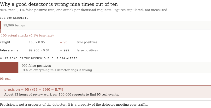
Ninety-one percent of everything this detector flags is wrong. If each alert costs a reviewer two minutes, this detector generates about 33 hours of review work per 100,000 requests to find 95 real events.
Precision is not a property of your detector. It is a property of your detector meeting your traffic. Vendor benchmarks are run on balanced sets, and your production traffic is not balanced.
This is why guardrail programmes fail socially before they fail technically. The alerts are mostly wrong, reviewers learn to dismiss them, and the queue becomes a formality. By the time a real event arrives, the muscle that was supposed to catch it has atrophied.
Three consequences for architecture:
- Know your base rate before you choose a threshold. If you do not know it, measuring it is the first piece of work, ahead of building the detector. Sample production traffic and label it.
- Reduce the population before you detect. Every deterministic filter that runs first shrinks the denominator. Entitlement checks at retrieval, format validation, and channel restrictions all raise the effective base rate for the expensive detector that runs after them. This is the strongest argument for the tiered design in ARCH-002.
- Do not send low-precision alerts to humans. Route them to an automatic mitigation that is cheap to be wrong about, such as redaction or an extra verification pass, and reserve human review for the high-precision band.
The threshold is a cost decision
A threshold is not a tuning parameter. It is an explicit statement about how much worse a missed attack is than a false alarm, and it should be signed off by whoever owns that risk rather than by whoever owns the model.
Write it down in that form:
  category:              pii_in_response
  cost(false negative):  regulatory disclosure, reportable
  cost(false positive):  one redacted field, user re-asks
  ratio:                 ~500:1
  implication:           tune for recall, accept low precision,
                         mitigate automatically rather than alert
category: block_user_request
cost(false negative): one attack proceeds to the next control
cost(false positive): legitimate user blocked, trust damage
ratio: ~1:20
implication: tune for precision, high threshold,
never the only controlBoth ratios above are illustrative, not benchmarks; the numbers that belong there are your own, and writing them down is the exercise.
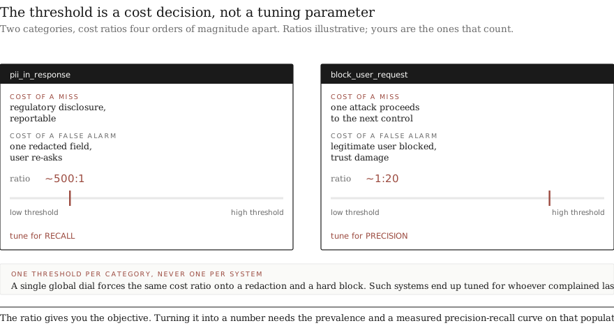
The ratio on its own does not give you a threshold. It gives you the objective. Turning it into a number needs two more things: the prevalence in the population the detector will run against, and a measured precision-recall curve for that detector on that population. With all three you can pick the operating point that minimises expected cost, and revisit it when the business context changes rather than when someone complains.
What a test set can support
Here is the discipline that separates a measured detector from a claimed one.
You hand-label 200 examples, run the detector, and report precision of 0.91.
The first thing to get right is which number is the sample size. Precision is measured over the items the detector flagged, not over the whole set. If those 200 examples produced 45 flags, your precision estimate rests on 45 observations, not 200, and its 95 percent interval is roughly 0.79 to 0.98. A competing detector that scored 0.88 on the same set is not distinguishable from it. Teams make that comparison on the point estimates and ship the loser.
Recall has the same problem with the other denominator: it rests on the number of actual positives in the set, which in a realistic sample of rare attacks is often a dozen or fewer. A recall figure computed from eleven true attacks should be reported as a range, and usually a range wide enough to be useless for ranking two detectors.
It gets sharper at the tail. To claim a false positive rate below some level, you need enough negative examples to have observed the absence. With zero false positives in n benign examples, the rule of three gives an upper bound of roughly 3/n at 95 percent confidence. So:
    100 clean, 0 false positives  ->  FPR could be as high as 3%
  1,000 clean, 0 false positives  ->  FPR could be as high as 0.3%
 10,000 clean, 0 false positives  ->  FPR could be as high as 0.03%
A team claiming a 0.1 percent false positive rate from a 500-example test set is claiming something their corpus cannot support. Given the base rate arithmetic above, the difference between 0.3 percent and 0.03 percent is the difference between a usable alert queue and an abandoned one.
Practical rules for the offline set:
- Label the negatives as carefully as the positives. Most effort goes into collecting attacks. Precision is determined by the benign class, and a benign set drawn from a different distribution than production makes the whole measurement fiction.
- Declare a label noise floor. Some fraction of your labels are wrong, and inter-annotator disagreement is the cheapest estimate of how large that fraction is. It does not impose a hard ceiling: a detector can legitimately exceed inter-annotator agreement, and disagreement can be resolved by adjudication. What it does mean is that differences smaller than the noise level are not interpretable, so a jump from 96 to 98.5 percent against a 4 percent disagreement rate is not evidence of an improvement. Report the disagreement rate next to the metric.
- Keep an untouched holdout. A test set that has been used to tune thresholds is a training set. Once you have iterated against it, it no longer estimates generalisation.
- Version the set. A metric that moves because the set changed, and one that moves because the detector changed, look identical in a dashboard.
Online validation
The offline set tells you how the detector behaves on the distribution you assembled. Production tells you how it behaves on the one you have. Three mechanisms, in the order you should build them:
Shadow mode. Run the detector on live traffic with its decisions recorded and not enforced. This is the only way to observe the real base rate and the real false positive volume before anyone is affected by it. Every detector should spend time here, and the exit criterion should be a number agreed in advance rather than a feeling that it looks fine.
Stratified sampling for labels. You cannot label everything. Sample deliberately across the score bands, oversampling the region near the threshold, because that is where the decisions are made and where your uncertainty is concentrated. Uniform random sampling spends almost all of its budget confirming that obvious negatives are negative.
The catch is that a stratified sample is no longer representative, so any population-level figure computed from it must be reweighted by the inverse of each band’s sampling rate. Skip the reweighting and you will report a precision that reflects your sampling design rather than your traffic, usually a pessimistic one, and the error is invisible in the dashboard.
A review queue that closes the loop. Human decisions on flagged items are a continuous source of fresh labels, already paid for by the review work itself. They become an asset only if the reviewer’s verdict is written back into a labelled store with the input, the detector version, and the evidence. Review workflows that discard this leave the programme starting each retraining cycle from nothing.
Two limits on that data. It is drawn entirely from items the detector flagged, so it can tell you about precision and can say nothing at all about false negatives. Measuring recall needs a separate sample of unflagged traffic, labelled independently, and that sample is pure cost with no operational by-product, which is why it is the first thing cut and the reason most guardrail programmes know their precision and merely assert their recall.
Regression discipline
Detectors are code and models, and both change. Treat the evaluation set as a test suite that runs in CI.
 on every change to a detector, ruleset, threshold, or model version:

   1  run the frozen regression set
   2  compare precision and recall per category vs the baseline
   3  fail the build on a drop beyond the agreed tolerance
   4  require an explicit, recorded override to ship a known regression
   5  record the new baseline only on a deliberate, approved change
Two additions that catch the failures a plain metric comparison misses:
A per-category breakdown, never an aggregate. An overall score that holds steady while one category collapses is the normal shape of a regression. Aggregates hide it by construction.
A canary set of previously-fixed false positives. Every false positive that gets fixed becomes a permanent test case. Without this, threshold tuning reintroduces old failures on a cycle, and the same complaint arrives from the same team twice a year.
The trigger for re-evaluation is not only a code change. Upstream model upgrades change the distribution of what your detectors see, and a prompt template change can shift the input distribution more than a detector change would. Both should fire the suite.
Where this blueprint stops working
Rare attacks resist measurement. For a category that occurs a handful of times a year, you will never assemble enough true positives to estimate recall. Synthetic attacks fill the gap and measure your ability to catch synthetic attacks, which is a different quantity. Be explicit about which categories are measured and which are asserted, and do not let the measured ones lend credibility to the rest.
Adversarial traffic is not stationary. Every metric here assumes tomorrow’s distribution resembles today’s. An adversary who learns your threshold invalidates that assumption deliberately. Metrics tell you about the attacks you have seen, and they are silent about the next class.
Human labels have a ceiling. Whether a given retrieval was a disclosure often depends on entitlement context the annotator does not have. Where the ground truth is genuinely contested, the honest move is to report the disagreement rate alongside the metric rather than resolve it by fiat and quote a clean number.